|
Raytracing Topics & Techniques - Part 4: Spatial Subdivisions by (26 October 2004) |
Return to The Archives |
Introduction
 |
|
The last scene from the previous article (the one with the sphere grid to show off the new refraction code) took almost 9 seconds to render on my pimpy 1.7Ghz Toshiba laptop with 1600x1200 screen (I know resolution has nothing to do with it, but I thought I would mention it anyway). And that's just for simple stuff. Later on we will add area lights, and to test the visibility of those, we will need lots of rays – for each pixel, that is. And, I would like to be able to render triangle meshes exported from 3DSMax, consisting of 10.000 triangles or more. That's going to take ages! It's easy to see what causes the delays: Every ray (primary and secondary) is intersected with about 100 spheres – Even if it's painfully clear that the ray doesn't hit the primitive by a long shot. In this article I will present some solutions for this. First, I will outline some algorithms, and then I'll explain how to implement a simple spatial subdivision scheme: The regular grid. And finally we'll have a look at performance improvements and some alternatives. |
|
Reducing Intersection Tests
|
|
A primary ray will hit only one primitive. In the raytracer that we built in the first three articles, this one primitive was found by trying them all, and keeping the closest one. This can take a lot of time if there are many primitives, and it's easy to see that rendering speed decreases linearly with the number of primitives in the scene. There are a couple of ways to make things better. |
|
Hierarchical Bounding Volumes
|
You could, for example group your objects, and encapsulate each group with a larger object (a sphere, or a box, for example). Now, if the ray misses the larger object, you can be sure it also missed the primitives in it. Storing multiple bounding volumes in an even larger volume reduces the number of tests even further. This is shown in figure 1: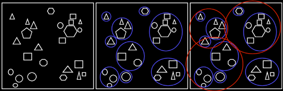 Fig 1: Hierarchical bounding volumes The first image shows a scene with quite a bit of detail. The second one shows the same scene, but this time groups of objects are encapsulated by bounding spheres. In the third image, groups of bounding spheres are grouped. When well executed, this technique can seriously improve rendering speed. The number of intersection tests is reduced to a fraction of the original count. There are however quite some cases where this algorithm will not perform so well. Looking at figure 1, it's easy to think up rays that hit several bounding spheres, but no primitives. And, in the above example you'll still need to test all three red spheres for every ray. Imagine a ray that hits the triangle in the upper left corner of the scene: The ray would first be tested against the three red spheres, then to the three blue spheres, and finally to the triangle. That's 7 tests. |
|
Use the GeForce, Luke
|
|
There is another way. Suppose you draw the scene using your favorite 3D accelerator. Each primitive is drawn using a unique color (which limits the number of primitives somewhat, but let's ignore that). Now, primary rays can be omitted completely: For each pixel, the raytracer merely reads the color value to identify which primitive is closest. The z-buffer can be used to determine the intersection point (although that's probably not very accurate). From there on, secondary rays can be spawned. This works quite well, especially when combined with the previous approach to accelerate the secondary rays. There's of course the limit to the number of primitives (not such a big problem when rendering to a 32bit target), and obviously you can't do supersampling like in the previous article. The biggest problem is obviously that this does not solve the problem for secondary rays, and once these start making up the majority of the spawned rays, you have to look for something else. |
|
Spatial Subdivisions
|
Have a look at figure 2: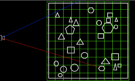 Figure 2: A regular grid This is the same scene as was used in figure 1, but this time it's subdivided by a regular grid. The camera in this image shoots two rays: The red one, and the blue one. Rays step through the grid, looking for primitives; as long as grid cells are empty, no intersection tests are performed. This means that the blue ray only tests one primitive. The red ray tests four primitives. That appears to be quite a bit better than the other algorithms. This algorithm has its problems too though: First, stepping through a regular grid is not very expensive, but not free either. Especially setting up the variables before the ray traversal starts can be quite costly. And, while in the above picture most cells only contain one primitive, this is obviously not always the case. And worse: Some cells may contain tons of primitives, while others are empty. An often used example is a football stadium with a highly detailed ball at the middle of the field. Storing this in a grid is a nightmare: There are lots of empty grid nodes, and then there is one grid node that contains the ball. Visiting this node means intersecting with all the triangles in it. Using a more detailed grid doesn't help (and if it does, we replace the ball with a detailed model of an ant). At the end of this article I will describe some algorithms that try to overcome these shortcomings. Despite the shortcomings, the regular gird performs quite well, and is reasonably easy to implement. I implemented the algorithm described in a paper titled "A Faster Voxel Traversal Algorithm for Ray Tracing" by Amanatides & Woo; a link to this paper is available at the end of this article. |
|
Grid Construction
|
|
First, the easy part. For the construction of the grid I have added a new primitive to scene.h / .cpp: An axis aligned box. This new primitive is used to represent cells in the grid, and also the bounding box of the grid. The implementation comes complete with an intersect method and normal calculation for the intersection point, so you can now add boxes to the scene. It's not very useful though, as you can't rotate the box: For the regular grid axis aligned boxes are sufficient. Note: Between writing this and sending it to Kurt, this got slightly changed; there is now an aabb class in common.h, which is used in turn by the Box primitive. The reason for this is that you don't want to attach a material etc. to a bounding box. Strictly, the Box primitive is no longer necessary, but I left it in as it's a nice change after all those stupid spheres. :) Next, all primitives now implement a new method: IntersectBox. This is used to determine whether or not a primitive is (partially) inside a cell of the grid. These are not terribly complicated; have a look at scene.cpp if you are curious. Now the grid can be constructed. This is done by the (new) BuildGrid method in scene.cpp. Initially this code looked like this:
For each cell, this code checks all primitives to see if they are in the cell or not. If they are, they are added to a list of objects, and a pointer to the list is added to the cell. This works fine for a couple of primitives, but when the number of primitives increases, it gets a bit slow: The code loops over all the primitives for each cell, and does an intersection test for each iteration. That's x * y * z * primitives intersections (i.e., a lot). The final version is faster:
This time the code first asks the primitive for it's axis-aligned bounding box, so that only the cells that could contain the primitive are checked. Note that this code also sets the extents of the grid. This is important, as rays won't be traced outside the grid. This does mean that a scene with an infinite ground plane suddenly won't be infinite anymore. |
|
Grid Traversal
|
|
Once the grid is constructed, we can start traversing it. This is done using a 3D version of the DDA algorithm. It works like this (the following is heavily based on the paper by Amanatides & Woo): First, we determine in which cell the ray starts. If the ray starts outside the grid, it must be advanced to a grid boundary; if it doesn't even hit the bounding box of the grid, obviously we are done with the ray. The coordinates of the first cell are stored in 'X', 'Y' and 'Z' (those are integers); we can use these coordinates to look up cells while traversing the grid. Next, we determine how far we can travel along the ray before hitting a cell boundary. We do this for the axii; the result is stored in tMaxX, tMaxY and tMaxZ. This is illustrated in figure 3: 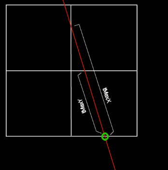 Fig. 3: tMaxX and tMaxY In this image, the ray is first advanced to the boundary of the grid (the green circle). From that point, we have to move 'tMaxX' to cross the vertical cell boundary, or tMaxY to cross the horizontal cell boundary. The minimum of these three values determines how far we can travel before we hit the first cell boundary. Finally, we determine how far we must move along the ray to cross one cell. Again, we do this for x, y and z; the result is stored in tDeltaX, tDeltaY and tDeltaZ. In the above image, tDeltaY equals tMaxY. Once we have the variables set up, we can start stepping through the grid. Stepping through the cells is illustrated in the following pseudocode:
In this code, stepX and stepY are used: stepX is set to '-1' if the sign of the x direction of the ray is negative, or 1 otherwise; stepY is calculated in the same way. The 3D version is a bit longer, but works in the same way. Have a look at the 'FindNearest' method in raytracer.cpp for the actual implementation. |
|
Processing Grid Cells
|
|
Each cell of the grid contains a pointer to a list of objects. Often, this pointer will be NULL, so no intersection tests will have to be performed. When a non-empty object list is encountered, the objects in the list are intersected. Take a look at the following situation: 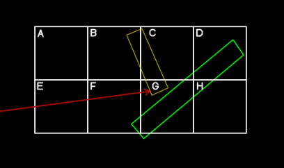 Fig. 4: Grid traversal problem In this example case, a ray enters the grid at cell 'E', advances to cell 'F' and intersects the rotated yellow rectangle in cell 'G'. Right, but first it will encounter the green rectangle, in cell 'F'. And it intersects this rectangle, although the intersection point is not inside cell 'F'. This problem could be solved by checking that intersection points are actually inside the cell that we are testing. But that's not a very nice solution: In the above example, the ray would miss the green rectangle in cell 'F', but it would test it again in cell 'G'. Two intersections for one primitive, that's not the way we want to go. |
|
Amanatides & Woo to the Rescue
|
|
The paper that I mentioned before presents a solution to this problem. First, the fact that the intersection is not occurring in the current cell is detected. While the intersection is outside the current cell, the ray is advanced to the next cell, and the objects in those subsequent cells are also tested. In the above case, this would mean that after finding an intersection (in cell 'H', but found while testing cell 'F') the algorithm will still check cells 'G' and 'H'. Multiple intersection tests are prevented by labeling the rays with a unique number, and storing this number during an intersection test, in the primitive. This way, when the same ray tries to intersect the same primitive again, this is easily detected, and the test is skipped. |
|
Implementation
|
| There are some more implementation details, but the basics of the algorithm should be pretty clear. The full implementation can be found in the 'FindNearest' method in raytracer.cpp. Full discussion of the algorithm is in the mentioned pdf. |
|
Performance Analysis
|
|
So how does it perform? You may be a bit disappointed to hear that the speed of the 'refraction scene' of the third article only doubled. At least initially I was disappointed. But it's not as bad as it looks: If you increase the complexity of the scene, the speed will not be affected very much, in contrast to the original approach. The following table shows this: 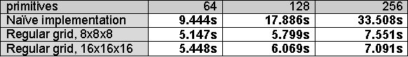 So, while it's only twice as fast at 64 primitives, it's three times faster at 128 primitives, and more than 4 times faster at 256 primitives. But why is it still so slow? The main reason for this is the expensive setup for the grid traversal algorithm: Intersecting a couple of spheres takes less time than setting up the variables. And, rays that start outside the grid must first be advanced to the boundaries of the grid. This requires a box intersection and adjusting the ray origin. This makes the startup cost for the regular grid traversal quite high. Stepping is not free either: Try increasing the grid resolution and you'll notice that speed drops even further. For complexer scenes this will probably be necessary; careful tweaking is recommended. 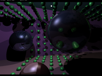 256 primitives in 7 seconds |
|
Alternatives
|
|
The regular grid is a rather simple spatial subdivision. Its regularity makes it easy to implement, and you don't have to take a lot of decisions when building the grid. Stepping is a bit complex but doable. Speed gain is OK. But isn't there anything better? Sure there is. Some alternatives: Nested grids: Imagine a grid cell that contains many primitives is subdivided in a grid. This would save many expensive intersection tests. And, it would let you use large empty cells in areas that contain little detail. Kd-trees: These seem to be the best choice at the moment for complex scenes. A Kd-tree is an axis-aligned BSP tree. What this means is that you start by splitting the scene bounding box along one axis. Next, you split both halves using the next axis. This process is repeated, using the three axii in turn. The position of the splitting plane can be specified; it's usually chosen in a way that balances the number of primitives to the left and the right of the plane, while minimizing primitive splits. A simpler version is the octree: In this version, you can't specify the position of the splitting plane; each cube is simply split in 8 equally sized cubes. As long as a cube contains more primitives than a certain threshold, cubes are split recursively. This results in large empty cubes for empty scene areas, and many smaller cubes for detailed areas. There are more spatial subdivision schemes, but these are the most well-known. |
|
Final Words
|
|
That's all for this article. The new gained performance paves the way for some new time consuming tricks, which I will discuss in the next article: Soft shadows and other effects that require lots of rays (but produce pretty pictures). By the way, if you improve the raytracer, please share your experiences and code! New primitives, cool scenes, speed enhancements are all welcome. If it's good stuff, I will add it to the raytracer and distribute it with the final package. Have fun, Jacco Bikker, a.k.a. "The Phantom" Links:
|